File:Conformal map.svg
Jump to navigation
Jump to search

Size of this PNG preview of this SVG file: 343 × 599 pixels. Other resolutions: 137 × 240 pixels | 275 × 480 pixels | 440 × 768 pixels | 587 × 1,024 pixels | 1,173 × 2,048 pixels | 2,287 × 3,991 pixels.
Original file (SVG file, nominally 2,287 × 3,991 pixels, file size: 2 KB)
Summary
| Description |
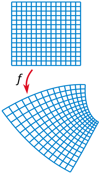
English: Illustration of a conformal map. |
| Date | |
| Source | Own work |
| Author | Oleg Alexandrov |
| SVG development |
Licensing
| This work has been released into the public domain by its author, Oleg Alexandrov. This applies worldwide. In some countries this may not be legally possible; if so: Oleg Alexandrov grants anyone the right to use this work for any purpose, without any conditions, unless such conditions are required by law. |
Source code
% Compute the image of a rectangular grid under a a conformal map.

function main()

   N = 15; % num of grid points
   epsilon = 0.1; % displacement for each small diffeomorphism
   num_comp = 10; % number of times the diffeomorphism is composed with itself

   S = linspace(-1, 1, N);

   [X, Y] = meshgrid(S);


   % graphing settings
   lw = 1.0;

   % KSmrq's colors
   red    = [0.867 0.06 0.14];
   blue   = [0, 129, 205]/256;
   green  = [0, 200,  70]/256;
   yellow = [254, 194,   0]/256;
   white = 0.99*[1, 1, 1];

   mycolor = blue;

   % start plotting
   figno=1; figure(figno); clf;

   shiftx = 0; shifty = 0; scale = 1;
   do_plot(X, Y, lw, figno, mycolor, shiftx, shifty, scale)

   I=sqrt(-1);
   Z = X+I*Y;

   % tweak these numbers for a pretty map
   z0 = 1+ 2*I;
   z1 = 0.1+ 0.2*I;
   z2 = 0.2+ 0.3*I;
   a = 0.01;
   b = 0.02;
   shiftx = 0.1; shifty = 1.2; scale = 1.4;
   F = (Z+z0).^2 +a*(Z+z1).^3 +b*(Z+z2).^4;
   F = (1+2*I)*F;

   XF = real(F); YF=imag(F);

   do_plot(XF, YF, lw, figno, mycolor, shiftx, shifty, scale)

   axis ([-1 1.3 -2 2]); axis off;

   saveas(gcf, 'Conformal_map.eps', 'psc2');


function do_plot(X, Y, lw, figno, mycolor, shiftx, shifty, scale)
   figure(figno); hold on;

   [M, N] = size(X);

   X = X - min(min(X));
   Y = Y - min(min(Y));

   a = max(max(max(abs(X))), max(max(abs(Y))));
   X = X/a; Y = Y/a;

   X = scale*(X-shiftx);
   Y = scale*(Y-shifty);

   for i=1:N
      plot(X(:, i), Y(:, i), 'linewidth', lw, 'color', mycolor);
      plot(X(i, :), Y(i, :), 'linewidth', lw, 'color', mycolor);
   end
%   axis([-1-small, 1+small, -1-small, 1+small]);
   axis equal; axis off;
File history
Click on a date/time to view the file as it appeared at that time.
| Date/Time | Thumbnail | Dimensions | User | Comment | |
|---|---|---|---|---|---|
| current | 03:48, 19 January 2025 | | 2,287 × 3,991 (2 KB) | wikimediacommons>Д.Ильин | Optimization |
File usage
The following 6 pages use this file: